

Large Language Models, or LLMs, drive much of what we see in today’s AI field. Most LLMs are built on Transformer architecture, which was first introduced in the “Attention is All You Need” paper. If you haven’t heard the story, this is the research that led to models like GPT, Llama, Gemini, and more broadly, almost every text generation model you see today.
But there’s a shift underway. The Diffusion method, which was originally used for image generation models like Stable Diffusion and DALL-E, is now starting to move beyond visuals. Text diffusion models are now emerging, and major players like Google are preparing to launch Gemini Diffusion, bringing diffusion techniques into the language space.
With this shift, it’s the right time to talk about how transformer models and diffusion models work in text generation, where they overlap, where they differ, and what the future might hold as these two approaches start to converge in generative AI.
Before we get into the topic, feel free to check some of my other AI articles you might find interesting.
The Current LLM Ecosystem
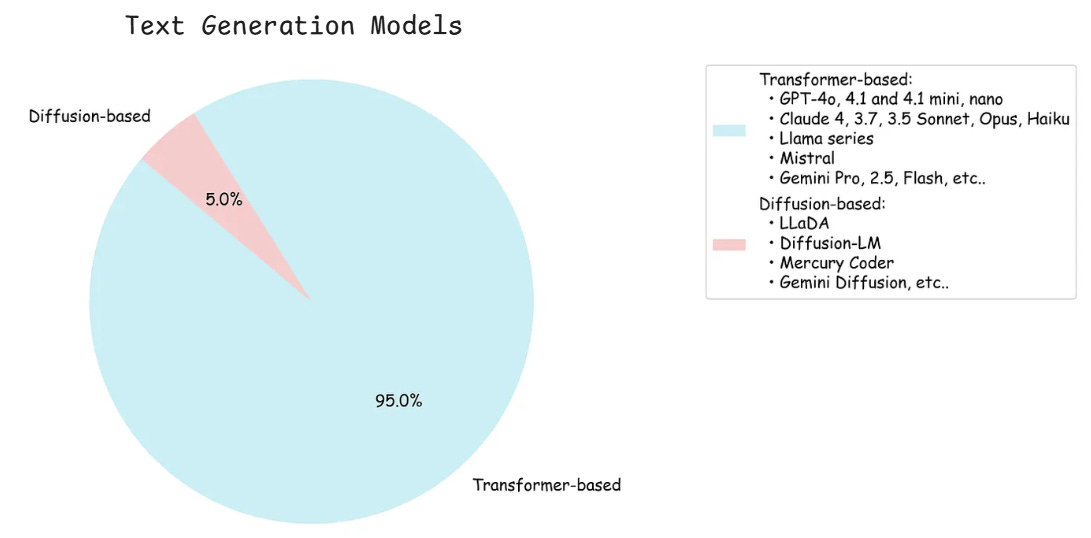
Here’s how today’s AI landscape looks when we break down available large language models by their core architecture. As we can see, Transformer models still dominate, but diffusion-based models are starting to appear.
Now let us understand how transformer-based models actually work.
How Transformer-Based LLMs Actually Work
All the popular LLMs today operate on the principle of next word prediction, powered by the Transformer architecture.
Video Source: Next Word Prediction with Transformer
In the video, "What date is it today?" prompt becomes a complete answer like "Today is Sunday.". Here's what's interesting; this entire response was built one token at a time, with each prediction feeding back into the system.
Each predicted word becomes part of the input for predicting the next word.
The cycle looks like this:
Input: "What date is today?" → Output: "Today"
Input: "What date is today? Today" → Output: "is"
Input: "What date is today? Today is" → Output: "Sunday"
And so on...
Each cycle uses the same internal process shown in the detailed diagram below.

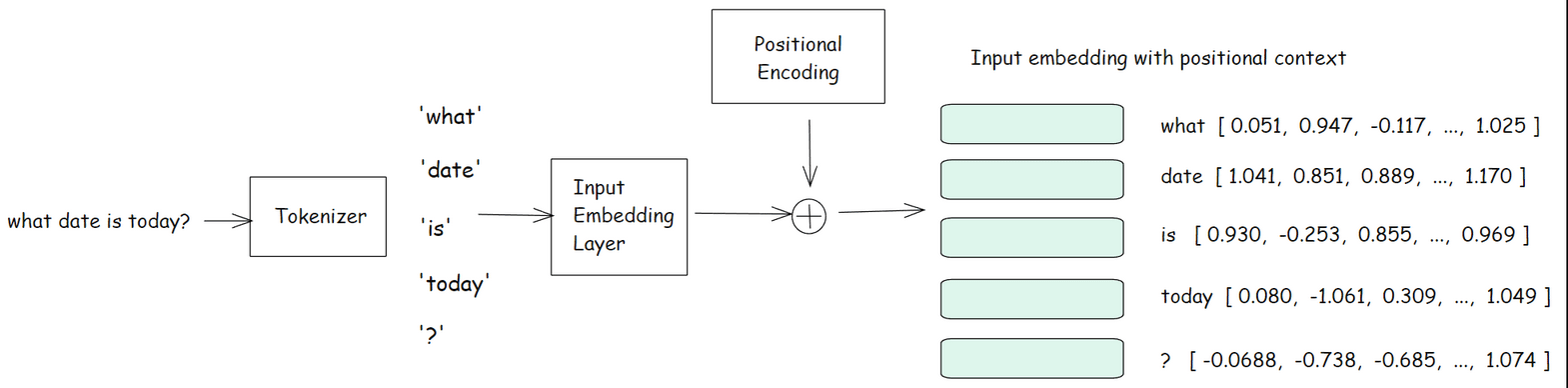
Now let’s break down the above diagram in detail. Below is the first half, which explains, how our input is turned into vector data. After the tokenizer converted the input into tokens (small words), the tokens are converted into embeddings (vector representation) along with the positional information.
Once we have these embeddings, they are fed into the Transformer block.
Let's see what's going on inside this Transformer block at a high level first, then we'll dive deeper into the details.

1. Multi Head Self Attention Mechanism:
The multi-head attention has several sub-steps that we need to understand. Let's go through each one.
Step 1.1: Turning Embeddings into Q, K, V Vectors
The very first operation inside the transformer specifically in Multi Head Attention block is to transform each of these incoming embeddings into three new vectors.
Query (Q)
Key (K)
Value (V)
This is done by multiplying each embedding with three different learned weight matrices (Query, Key, Value).
For example, for the token "what," we will get Q_what, K_what, V_what.
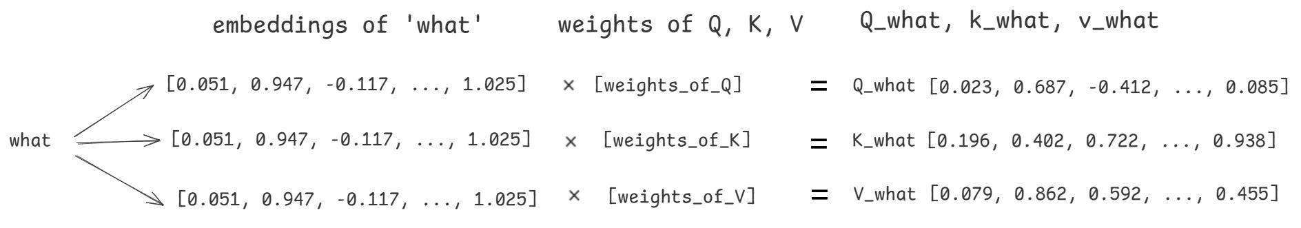
Q_what: What information “what” is looking for from other tokens.
K_what: What information “what” has to offer to other tokens.
V_what: The actual information of “what”.
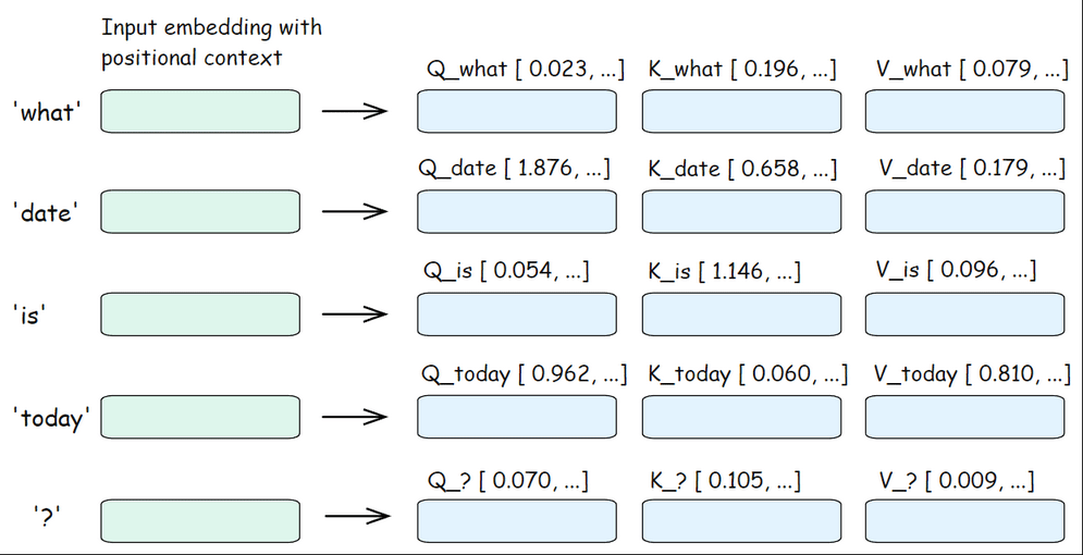
This process happens for every token in the input. So, we will have Q, K, V Vector for every token.
With the Q, K, and V vectors ready for all tokens, the model can now start figuring out which tokens are important to each other. This is known as self-attention process.
Step 1.2: Calculating Attention Scores
In this step, each token uses its Q, K, and V vectors to determine how much attention it should pay to every other token in the sentence. This is what makes transformers so powerful at handling context.
How does this work?
For every token, its Query (Q) is compared with the Keys (K) of all other tokens in the sentence, including itself.
This comparison is done using a dot product which is a way to measure similarity between two vectors. Q × K calculates which tokens are most relevant to the current token.
To keep things stable, we divide by the square root of the vector size.
The formula looks like this:
Attention Score = Q × Kᵀ / sqrt(dim)Q: The query vector for the current token.
Kᵀ: The transposed key vectors of all tokens.
dim: The size of the key/query vectors.
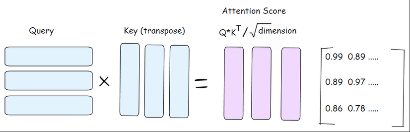
What does this mean in practice?
A higher score means the current token finds that other token more relevant or important for the next prediction. The result is an attention score matrix, a grid that shows, for every word, how much it "cares about" every other word.
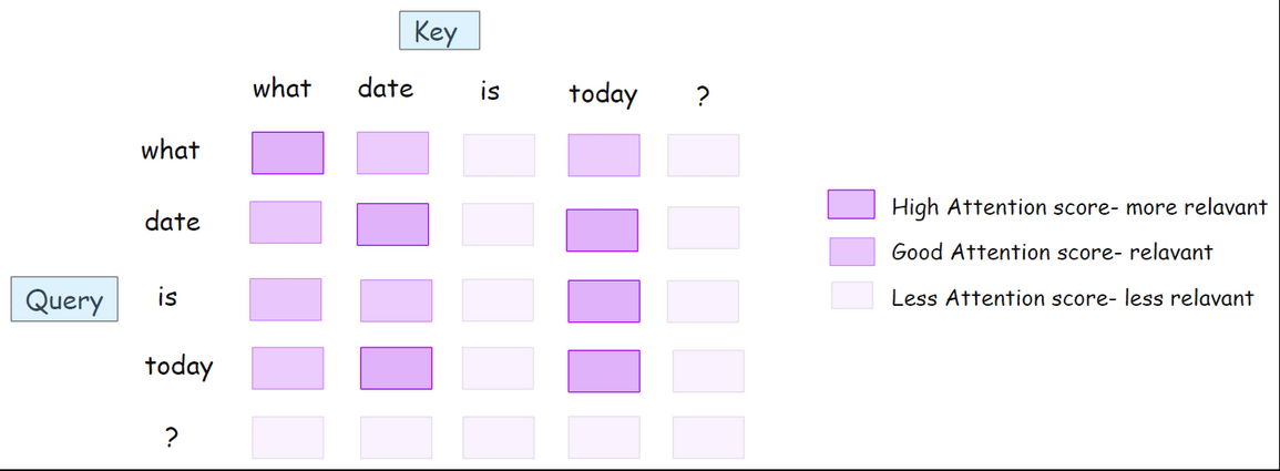
Example Attention Score Matrix for our sentence:
Attention Score Matrix (5×5):
          what   date   is     today   ?
what      0.99   0.89   0.12   0.88   0.34
date      0.89   0.97   0.23   0.95   0.26
is        0.86   0.78   0.15   0.87   0.12
today     0.67   0.95   0.14   0.98   0.23
?         0.13   0.15   0.02   0.14   0.09
So, for example, "what" pays the most attention to itself, then to "date" and "today, just as highlighted in the diagram below.
Step 1.3: Masking
Before turning attention scores into probabilities, the model needs to make sure it can’t “peek” at any words that come after the current one. To do this, it applies a mask. All attention scores for future tokens are set to negative infinity. When these masked scores go through the SoftMax step, their probabilities become zero.
This ensures that the model gives zero attention to future tokens and pays attention only to the current and previous tokens.
For example, when the attention score for the word "date" is being calculated, it's important that "date" doesn't get a look at "today", which is a future word in the sequence. Masking happens because the model was trained to process text left-to-right, one word at a time.
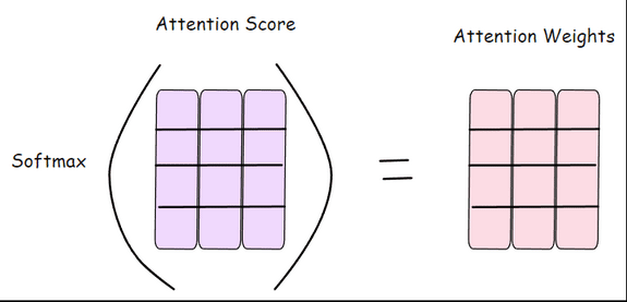
Step 1.4: Turning Attention Scores into Weights (SoftMax)
The attention scores tell us which words are most relevant, but at first, they're just plain numbers. To make them useful, the model runs each row through something called a SoftMax function. This changes the scores into probabilities between 0 and 1, so the model knows exactly how much attention to give each token.
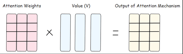
Step 1.5: Mixing With the Value Vectors (Building Context)
Now we use the attention weights to create the output of multi-head attention. Each token takes the Value vectors from all other tokens and mixes them based on the attention weights.
How does it work,
High attention weight = take more information from that token's Value vector
Low attention weight = take less information from that token's Value vector
Zero attention weight = ignore that token's information completely
For example, if "what" has high attention weights for "date" and "today", it will mostly use information from "V_date" and "V_today" to build its final representation.
So far, we’ve described this attention process for a single head. But transformers use multiple heads simultaneously. Each head learns to focus on different patterns in the sentence, and their outputs are combined to give the model a richer understanding of the context.
2. Add & Normalization
After multi-head attention, the transformer does two quick things to maintain stable learning.
Add (Residual Connection): The original input gets added back to the output of multi-head attention. This is called a residual connection and helps the model keep track of the original information.
Normalize: Then, the result goes through a normalization layer called LayerNorm to keep the values stable for better learning.
3. Feed-Forward Neural Network
After Add & Normalize, the output flows into a feed-forward network. This part is basically a mini neural network. It consists of two linear layers separated by an activation function. The data gets expanded, transformed, and compressed back, helping the model capture more complex patterns and relationships.
4. Add & Normalize (again)
After the feed-forward network, the model repeats the same Add & Normalize step, just like it did after multi-head attention. This input to the feed-forward part is added back to its output (residual connection), and then the result is normalized (LayerNorm). Doing this again helps keep the data stable and learning smooth as it moves through the transformer layers.
To better understand steps 2, 3, and 4, here's the diagram again with the Add & Normalization blocks highlighted, along with the Feed Forward Network in the middle.

5. Output Layer
After the data has moved through all the transformer layers, we end up with a set of context-rich vectors, one for each token. But the job isn’t finished yet, the model still needs to generate the output token one by one. Here comes the output layer.
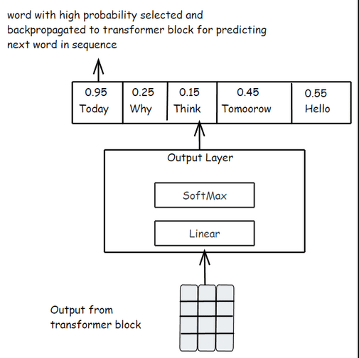
Step 5.1: Linear Layer:
Each token’s final vector is passed through a linear layer, which transforms it into a vector as long as the model’s vocabulary. For example, if the model knows 50,000 words, the output will be a vector with 50,000 values, one for each possible next word. For example, GPT-3's vocabulary is 50,257 tokens, so the output will be a vector with 50,257 values.
Logits:
The values in this output vector are called logits. Each logit represents how likely the model thinks a specific token could be the next word.
Step 5.2: SoftMax Function:
The logits go through a SoftMax function, which converts them into probabilities between 0 and 1. Now, we have a probability distribution over every possible word in the vocabulary.
Selecting the Next Token:
Usually, the token with the highest probability is chosen as the next word.
A Note on Transformer Architectures: Encoder, Decoder, or Both?
Up to this point, we’ve walked through the full flow of a single transformer block, showing how an input sequence gets embedded, passes through self-attention and feed-forward layers, and finally predicts the next word. But depending on the use case, not every transformer model is built exactly the same way.
There are three main ways transformer architectures are used.
Encoder only
Decoder only
Encoder-Decoder Model
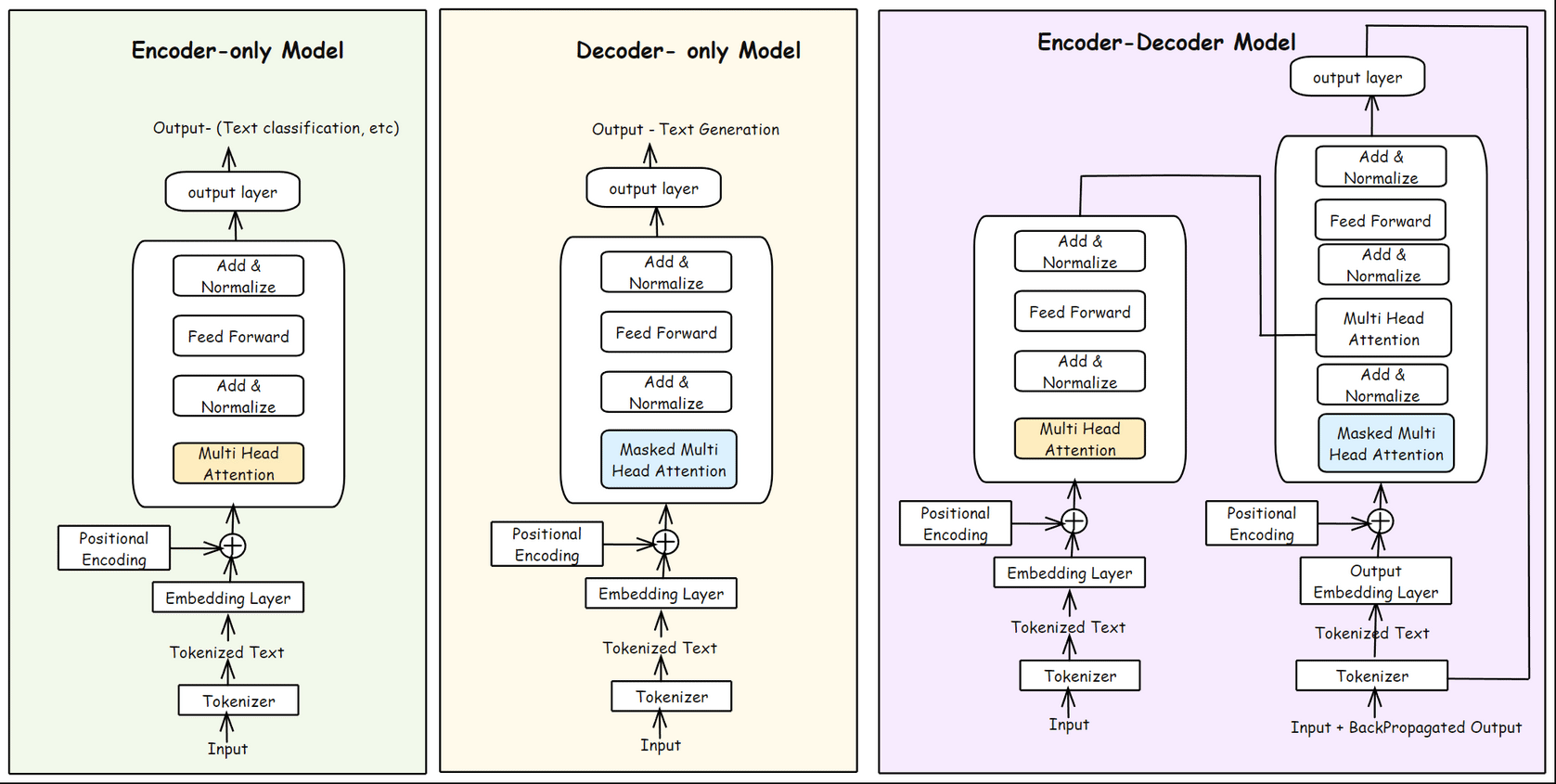
As we can see, encoder-only models stack just the encoder blocks while decoder-only models stack only the decoder blocks which include masked self-attention to prevent the model from peeking ahead. Encoder-decoder models combine both, the encoder processes the input, and the decoder generates output one step at a time, attending to both its own previous outputs and the encoder’s representations.
Encoder-Only Models:
Models like BERT, use just the encoder stack. They’re designed for understanding input text. These models are built for tasks like classification, sentence embedding, or question answering where we want to deeply analyze and represent the meaning of an input.
Encoders are built to create rich vector representations (“embeddings”) of input text, which can then be used for tasks like classification, similarity matching, or extracting key information.
Example: BERT, RoBERTa, DistilBERT,
Decoder-Only Models:
Models, like GPT and Llama, use only the decoder part of the transformer. They focus on generating text, predicting the next word one at a time, making them ideal for text generation, completion, and conversation.
Example: GPT series, Llama, Mistral,
Decoders are designed to generate new texts. For example, answering user queries or text completions.
Encoder-Decoder Models:
This is the original transformer setup from the “Attention is All You Need” paper. Here, the encoder reads and encodes the entire input sequence into context-rich representations, and the decoder generates the output sequence step-by-step.
Example: T5,
In summary:
Encoder-only: Text understanding
Decoder-only: Text generation
Encoder-Decoder: Translation and summarization
Where Does Our Example Fit?
The step-by-step transformer workflow we described in this blog most closely follows the “decoder-only” setup used by large language models like GPT and Llama, where the model generates one token at a time.
But under the hood, all three architectures use the same building blocks multi-head self-attention, residual connections, normalization, and feed-forward networks.
This video shows how the model picks the next word and how the temperature setting changes which word gets chosen. Temperature modifies the logits before applying the SoftMax function, which is why changing it can make the predictions either more focused or more creative.
At this point, we've taken a deep dive into how transformers work and the variety of architectures. The highlight is their ability to capture complex relationships and context, no matter how long the sentence, by letting every word pay attention to every other word in the sequence. That’s why transformers form the backbone of almost every state-of-the-art text model we see today.
But transformer-based models aren’t the only ones in town.
Enter Diffusion Models…
Diffusion Models
Before transformers took over, the idea for diffusion models was introduced back in 2015 by researchers inspired by physics. The key idea is to take real data, like an image or a sentence, add noise step by step until it’s completely scrambled, then teach a model to reverse the process and recover the original data.
Diffusion models work very differently from transformers. Instead of building things one step at a time, they start with pure noise and learn to gradually clean it up, producing meaningful results along the way. These models first became famous for generating images, but now they’re starting to make an impact in text generation too.
Over the past few years, diffusion models have rapidly evolved. The field started with basic DPMs (Diffusion Probabilistic Models) in 2015 and has since seen a wave of breakthroughs from DDPMs and DDIM, to more recent text-focused models like Diffusion-LM, DiffuSeq, LLaDA, Mercury Coder. The progress has been fast, as we can see in the timeline below.
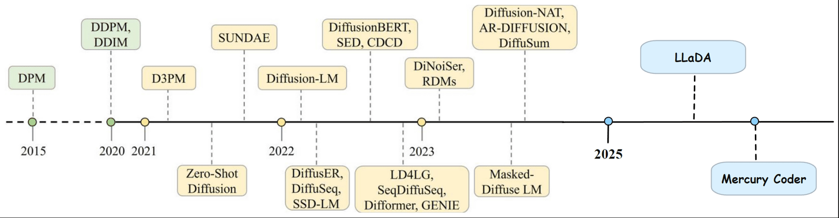
Denoising Diffusion Probabilistic Models (DDPMs) were among the first diffusion models to gain widespread attention. They use a diffusion process, where noise is added and then removed step by step, making the process relatively simple to implement and train.
New architectures and training strategies have pushed diffusion models beyond images into text, code, and even more complex generative tasks. In 2025, models like LLaDA and Mercury Coder are leading the way in diffusion-based language modeling, showing just how far this technology has come.
How Diffusion-Based LLMs Generate Text
As already mentioned above, diffusion models don’t generate one token at a time, they start with a noisy, partially masked version of the output and progressively denoise it by refining the entire sequence in parallel, until a clean, coherent sentence arrives.
Let’s break down this process.
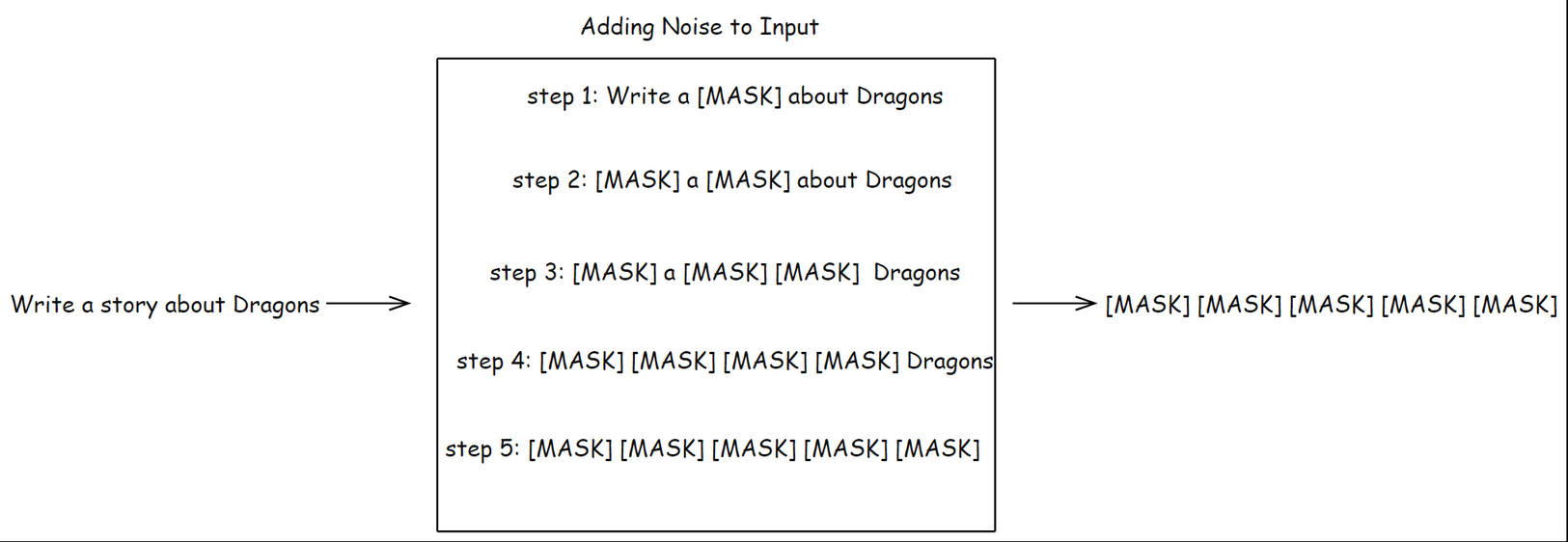
1. Forward Process: Adding Noise to Text
During training, the model takes a real text sequence and gradually adds noise, or masks out tokens, step by step. The amount of corruption at each step is controlled by a noise or mask schedule.
In LLaDA: This is done by randomly masking tokens throughout the sentence, increasing the mask ratio as steps progress.
In Mercury Coder: The noise can be added directly in embedding space, and entire token embeddings can be corrupted in parallel.
By the end of this process, the original sentence is almost unrecognizable either mostly masked out or replaced by noisy embeddings.
2. Training: Learning to Denoise
The core challenge is to train the model to reverse the corruption. At every denoising step, the model (usually a transformer or U-Net backbone) receives a partially masked (or noisy) sequence and is asked to predict what the less-corrupted version should look like.
For example, if given:
Noisy input: "[MASK] [MASK] story [MASK] dragons"
Target: "Write a story about dragons"
The model learns to fill in the [MASK] tokens with the correct words. It does this for thousands of examples, learning patterns of how to denoise text at every corruption level.
Training Objective
The model learns by practicing how to clean up noisy text. During training, it gets shown text with different amounts of noise added and tries to guess what the original clean text was. The model gets better by comparing its guesses to the correct answers and adjusting when it's wrong. By practicing with lots of different noise levels, it learns to fix text no matter how noisy it is.
3. Text Generation Flow: Using Learned Denoising
At inference time, the process runs in reverse.

Fixed-length parallel generation: The model starts with a fully masked sequence of predetermined length and denoises all positions simultaneously, not word-by-word like transformers.
Multi-step refinement: The denoising happens gradually over multiple steps (typically 10-50+ steps), with each step refining the predictions across the entire sequence.
Mask-to-text prediction: At each denoising step, the model predicts which tokens or embeddings should replace the current noise/masks, progressively revealing coherent text.
Parallel processing advantage: Unlike sequential generation, all token positions are refined together in each step, enabling faster generation in models like Mercury Coder.
This process continues until the sequence is fully denoised, resulting in a coherent, meaningful text output.
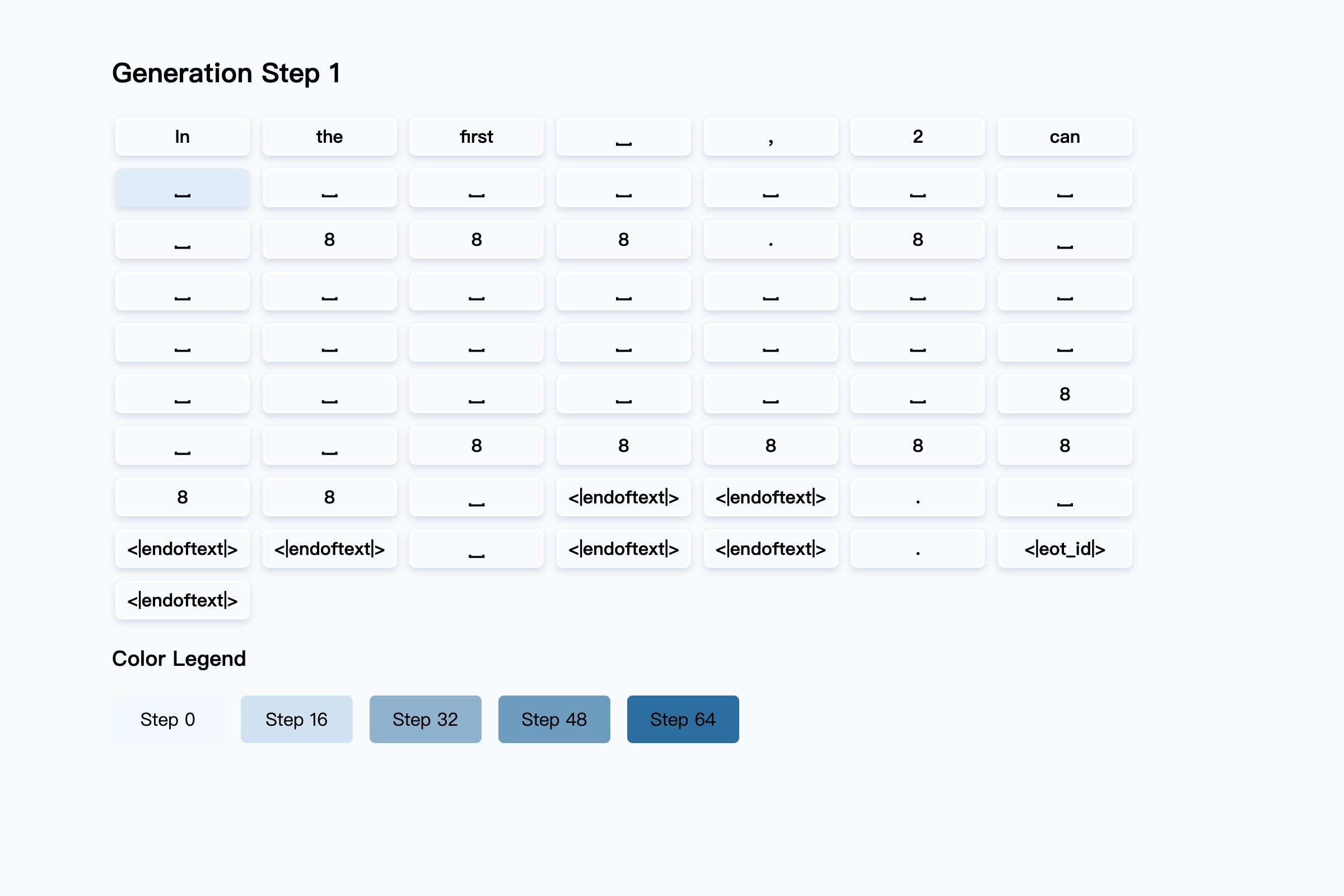
Want to see what this process looks like in action?
Unlike transformers, which generate one token at a time, diffusion LLMs fill in many words at each step, gradually building up the final answer. The diagram below shows how diffusion model responds to a user question gets constructed over several rounds. Darker colors show tokens filled in during the later stages, while lighter colors are guessed earlier in the process.
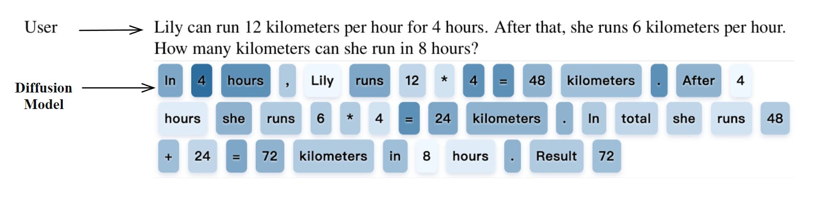
See how it is achieved in total of 64 steps…
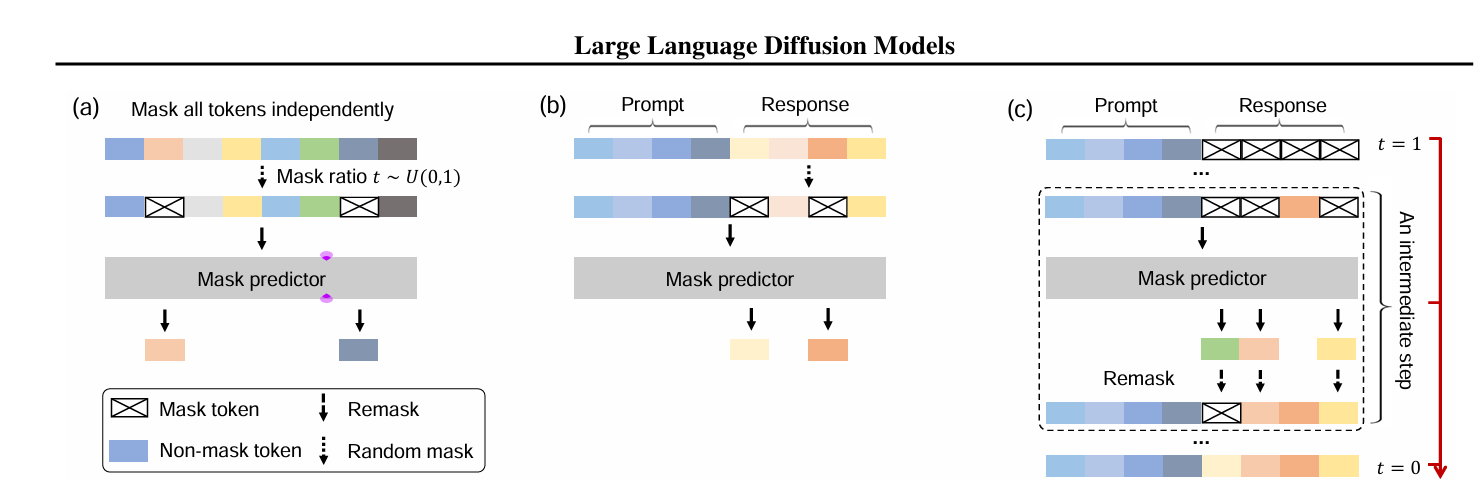
Here’s a visual overview of how the LLaDA diffusion language model works:
(a) Pre-training: The model takes real text and randomly masks tokens at different positions. Its job is to predict the original values for the masked tokens, learning to fill in blanks no matter where they appear.
(b) Supervised Fine-Tuning: When fine-tuning for tasks like question-answering, only the answer part is masked, and the model learns to reconstruct it given the full prompt.
(c) Generation (Sampling): To generate new text, LLaDA starts with a fully masked response and then, in several steps, predicts some tokens and unmasks them, repeating until all tokens are filled in. This re-masking and prediction are what allows the model to go from pure noise to a meaningful answer.
What Makes Diffusion LLMs Unique?
Global, Bidirectional Context: At every step, the model can look at all positions in the sequence (both left and right), so it captures dependencies across the entire sentence, not just one direction. This helps with tasks like reasoning and code completion where context matters everywhere.
Parallel Generation: Unlike autoregressive transformers, which generate text one token at a time, diffusion LLMs update many tokens at once, enabling much faster inference, especially on GPUs.
Strong Performance: As shown in models like Mercury Coder and LLaDA, diffusion LLMs can match or outperform traditional LLMs on standard language and coding benchmarks, while being more efficient.
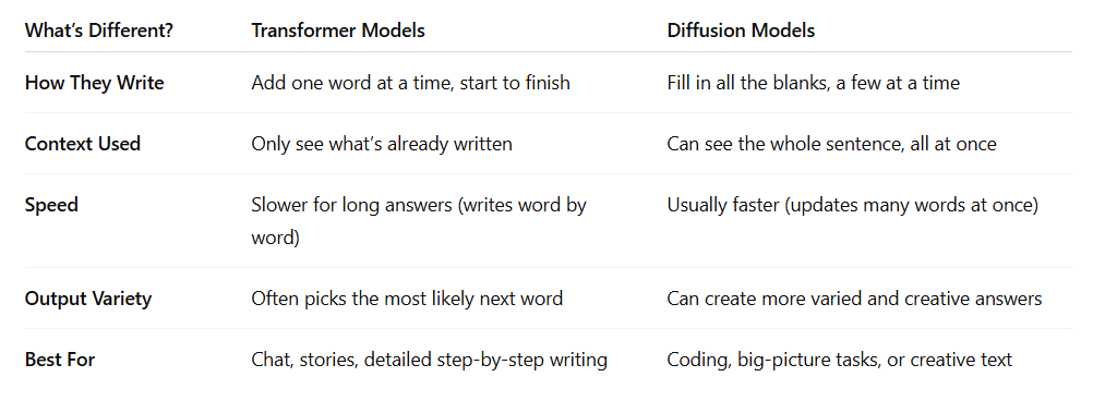
A comparison: Transformer Vs Diffusion Method
Final Thoughts
We’ve covered a lot, from how transformers became the foundation for most of today’s text generation models, to how diffusion methods are now bringing something fresh to the table. It’s amazing to see how far things have come in just a few years.
With models like LLaDA and Mercury Coder leading the way, and Google set to release Gemini Diffusion, it feels like we’re at the start of another big shift in AI. It’ll be exciting to see how diffusion-based language models stack up as they hit the mainstream.
References taken for Transformer and Diffusion Models:
I hope you enjoyed this blog!
Until we meet with the next piece, Happy Learning!